Observability has always been directly linked to reliability in distributed systems. After all, it’s hard to reason about things you can not see. Thanks in part to Google’s espousal of Site Reliability Engineering principles (the SRE Bible has been a free read on-line for awhile now, so go check that out if you haven’t yet!), the continuous evolution of our craft, and an abundance of cloud native tooling… observing value-producing things is easier than ever.

Unfortunately, a well-tuned observability platform closely integrated with a large infrastructure often presents enough complexity as a whole that it may look like magic. In reality, it is a number of purpose-built and thoughtfully-selected components used with intent.

A recent refactoring effort led me to modernize a smoketest framework I built for Cloud Foundry service instances. When originally designed, my primary focus was exposing various aspects of the systems under test via API endpoint. The idea was for upstream pipelines or monitoring systems to consume the API and extract useful data. Here’s an example of JSON data returned during normal operation:

    "results": [
        {
            "instance": "my-mongodb",
            "message": "OK",
            "secondsElapsed": 0.172
        },
        {
            "instance": "my-mysql",
            "message": "OK",
            "secondsElapsed": 0.069
        },
        {
            "instance": "my-postgres",
            "message": "OK",
            "secondsElapsed": 0.057
        },
        {
            "instance": "my-rabbitmq",
            "message": "OK",
            "secondsElapsed": 0.065
        },
        {
            "instance": "my-redis",
            "message": "OK",
            "secondsElapsed": 0.092
        }
    ]
}

Each test performs a number of CRUD operations against the configured service instance, and reports timing. Error messages bubble up along with non-200 HTTP status codes. Together, this allows trending of error rate and latency from the four golden signals.

While this worked, it required additional integration effort to provide value. At the time I focused on figuring out how to test each of the service types and didn’t think about upstream instrumentation. Since then, Prometheus has become a ubiquitous choice for observability.

Thankfully, Prometheus has a large number of battle-hardened client libraries. Simply pick one for your favorite language, and start instrumenting. Each has a familiar look and feel. Import the library, do some baseline configuration (such as polling interval and metric prefix for default metrics, and whether or not you even emit default metrics), expose a /metrics endpoint, and define SLIs you care about. We’ll walk through each of these steps in a simple Node.js app below.

SLI — a carefully defined quantitative measure of some aspect of the level of service that is provided.

Getting Started

Getting started with Prometheus is easier than you think. All code examples will be fully functional, but to reduce noise I’m going to trim surrounding bits where it makes sense. If you are curious about the bigger picture, be sure to check out the project repository.

Before we can do anything useful, we need to import the client library and expose a /metrics endpoint. If you followed the client library link above, you probably came across the most popular community option for Node.js (prom-client). Here’s how we leverage prom-client with Node.js and Express:

const prometheus = require('prom-client')

prometheus.collectDefaultMetrics({ prefix: 'splinter_' })

app.get('/metrics', (req, res) => {
  res.set('Content-Type', prometheus.register.contentType)
  res.end(prometheus.register.metrics())
})

The second line is entirely optional, and simply configures a prefix for the default metrics emitted by Prometheus. These give you useful signals about the health of your runtime environment out of the box. If you want to disable them, you can simply add a couple more lines of code:

clearInterval(client.collectDefaultMetrics());
client.register.clear();

That’s it! You have a metrics endpoint exporting any registered metrics… so let’s go define some of those now.

Defining Metrics

Prometheus supports a number of metric types to provide flexibility. The key is picking the right metric type for your use case. Common choices include:

Counters: Track the number or size of events. Typically used to track how often a particular code path is executed.

Gauges: Snapshot of current state. Unlike counters, gauges go up and down to reflect the measured value over time.

Summaries: Like a timer, but can grow (positively) by any amount and average results.

Histograms: A familiar bucketed metric lending itself to quantiles and percentiles.

Thinking back to the golden signals discussed above, counters are particularly useful for calculating things like error rate. Percentiles are a good match when reasoning about latency or throughput, and how performance fits within our SLOs.

SLO – A target value or range of values for a service level that is measured by an SLI.

Selecting the right types of metrics is much like choosing the right bread for a sandwich… A wrong choice will likely lead to unsatisfying results no matter how much effort you invest elsewhere. While summaries look like a good fit in many cases, one caveat to be aware of is summaries can not be aggregated. Read this to better understand the trade-offs when comparing summaries and histograms.

To calculate error rate, we actually need two counters (one for total requests, and one for errors). For latency, we only need a single histogram. While histograms are flexible (you can define custom buckets and labels), luckily the default case works well for web services (covering a range of latencies from 1 millisecond to 10 seconds). Here’s what we need for one of our test cases:

const prometheus = require('prom-client')

const requestsMongodb = new prometheus.Counter({
  name: 'splinter_mongodb_tests_total',
  help: 'Total MongoDB tests across process lifetime.',
})

const errorsMongodb = new prometheus.Counter({
  name: 'splinter_mongodb_errors_total',
  help: 'Total MongoDB errors across process lifetime.',
})

const latencyMongodb = new prometheus.Histogram({
  name: 'splinter_mongodb_latency_seconds',
  help: 'MongoDB test latency.',
})

module.exports = {
  requests: requestsMongodb,
  errors: errorsMongodb,
  latency: latencyMongodb,
}

Instrumentation

The next step is actually instrumenting our code. This involves incrementing counters after key events, and observing results for histogram bucketing. Assuming we’ve defined and exported the metrics we defined above, that boils down to just a few lines:

const { requests, errors, latency } = require('../metrics/mongodb')

try {
    // success
    requests.inc()
    latency.observe(testState.results.secondsElapsed)
} catch (error) {
    // fail
    errors.inc()
}

Quick and easy! At this point, running our app will nicely collect success, error and latency metrics on each transaction. It will expose these in Prometheus exposition format via our /metrics endpoint. In the example below, I’ve generated some test traffic… Note how our histogram provided a range of buckets convenient for SLO calculations, even with minimal configuration on our part:

# HELP splinter_mongodb_tests_total Total MongoDB tests across process lifetime.
# TYPE splinter_mongodb_tests_total counter
splinter_mongodb_tests_total 1029

# HELP splinter_mongodb_errors_total Total MongoDB errors across process lifetime.
# TYPE splinter_mongodb_errors_total counter
splinter_mongodb_errors_total 0

# HELP splinter_mongodb_latency_seconds MongoDB test latency.
# TYPE splinter_mongodb_latency_seconds histogram
splinter_mongodb_latency_seconds_bucket{le="0.005"} 0
splinter_mongodb_latency_seconds_bucket{le="0.01"} 0
splinter_mongodb_latency_seconds_bucket{le="0.025"} 9
splinter_mongodb_latency_seconds_bucket{le="0.05"} 703
splinter_mongodb_latency_seconds_bucket{le="0.1"} 902
splinter_mongodb_latency_seconds_bucket{le="0.25"} 1014
splinter_mongodb_latency_seconds_bucket{le="0.5"} 1028
splinter_mongodb_latency_seconds_bucket{le="1"} 1029
splinter_mongodb_latency_seconds_bucket{le="2.5"} 1029
splinter_mongodb_latency_seconds_bucket{le="5"} 1029
splinter_mongodb_latency_seconds_bucket{le="10"} 1029
splinter_mongodb_latency_seconds_bucket{le="+Inf"} 1029
splinter_mongodb_latency_seconds_sum 60.257999999999825
splinter_mongodb_latency_seconds_count 1029

Visualization

While we’re headed in the right direction, staring at metrics endpoints is not the end goal. Modern teams typically have dashboards to help visualize key metrics they care about. There are two common ways to visualize metrics generated by Prometheus.

The first is the Prometheus Expression Browser. This is useful as an exploratory tool, letting you experiment with PromQL queries which are flexible and expressive enough it can take time to find the right incantation. In its simplest form, all you need is a local Prometheus and simple scrape configuration pointed to your metrics endpoint. This is where the simplicity of Prometheus really shines, letting you quickly fire it up most anywhere during development:

brew install prometheus

cat <<EOF
global:
  scrape_interval: 10s
scrape_configs:
  - job_name: splinter
    static_configs:
      - targets:
        - splinter.cfapps.io:80
EOF

./prometheus

By default, the Prometheus process will listen on localhost:9090 and serve the Expression Browser under /graph (the root path will redirect). You can see how Prometheus has already discovered the metrics emitted by our application:

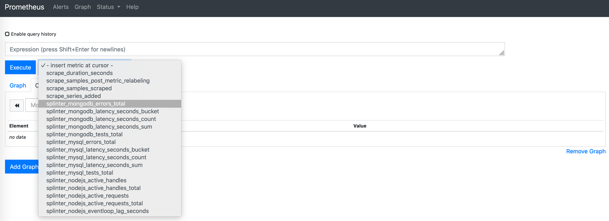
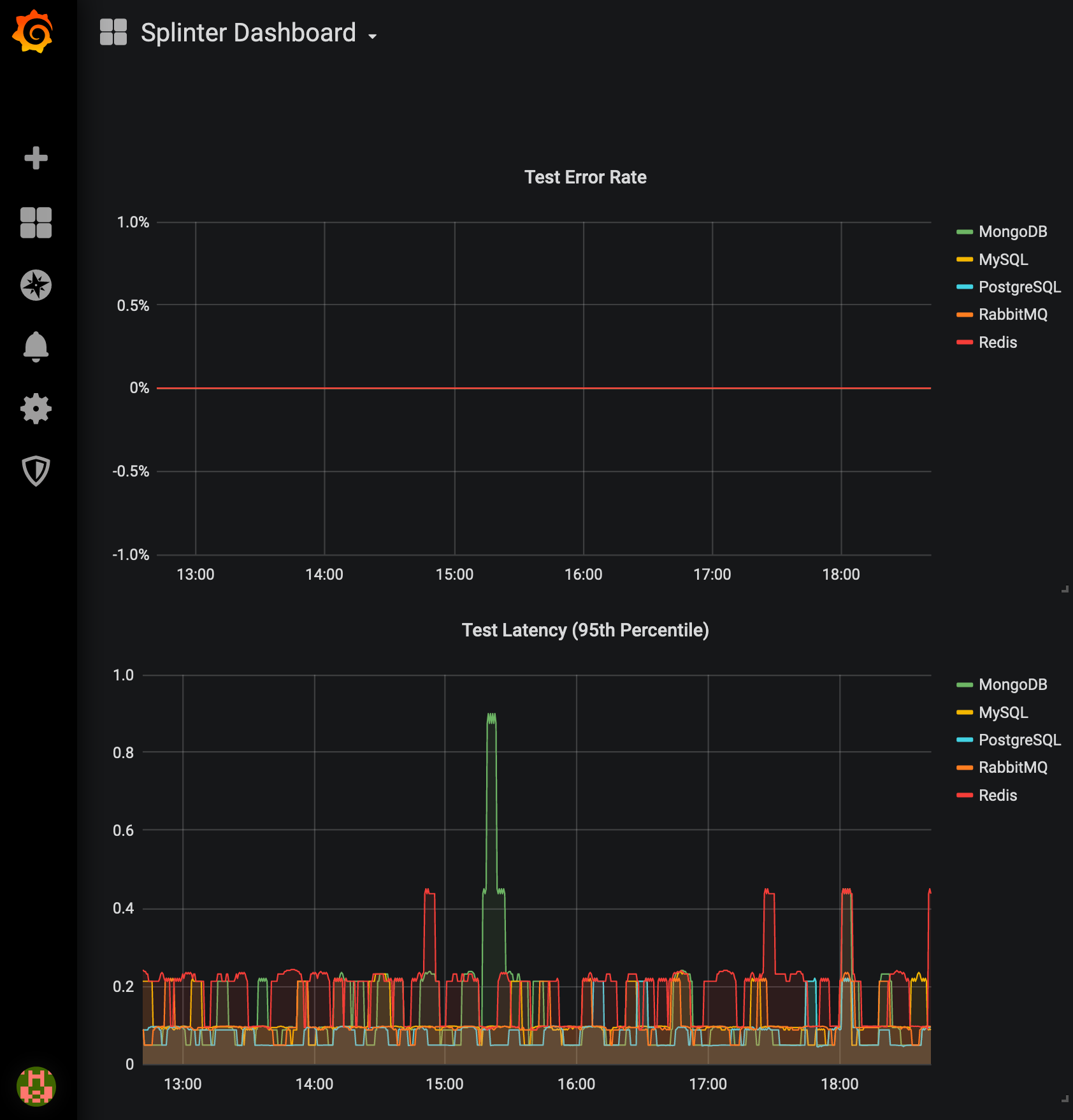
You can plot individual metrics by selecting them and clicking Execute, or piece together more powerful queries. In our case, we are interested in two queries for each set of metrics emitted by our tests… Error rate:

rate(splinter_mongodb_errors_total[5m]) / rate(splinter_mongodb_tests_total[5m])

And 95th percentile latency:

histogram_quantile(0.95, rate(splinter_mongodb_latency_seconds_bucket[5m]))

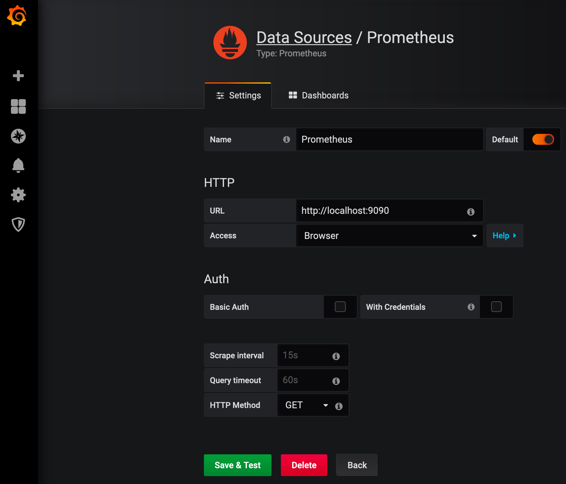
Almost there…  we’ve explored enough to find good starter queries. The final step is integrating with a visualization tool for dashboarding. Grafana has become as ubiquitous as Prometheus, evolved to support a variety of common data sources, and looks great to boot. Configuring Grafana to work with Prometheus is straightforward:

• Install Grafana (for development you can just fire up a Docker container)
• Install and configure a Prometheus data source
• Add graph panels leveraging the queries you discovered above
• Tweak visualization options to meet your needs

Conclusion

In the real world your application will be more complicated. It will need to fit into a larger ecosystem. You will also need to put more thought into how Prometheus itself is deployed, and what visualization technology you select. The good news is, none of this is magic. Good opensource tools exist to solve your observability problems, regardless of your architecture or language of choice. The instrumentation itself is lightweight, flexible and easy to implement incrementally. Go forth and visualize!

For a quick developer-friendly guide to getting Prometheus and Grafana up and running against your instrumented application, including a dashboard template, check this out.

Thanks for reading!